K-Tensors – Clustering Positive Semi-Definite Matrices
Functional Connectivity Matrix

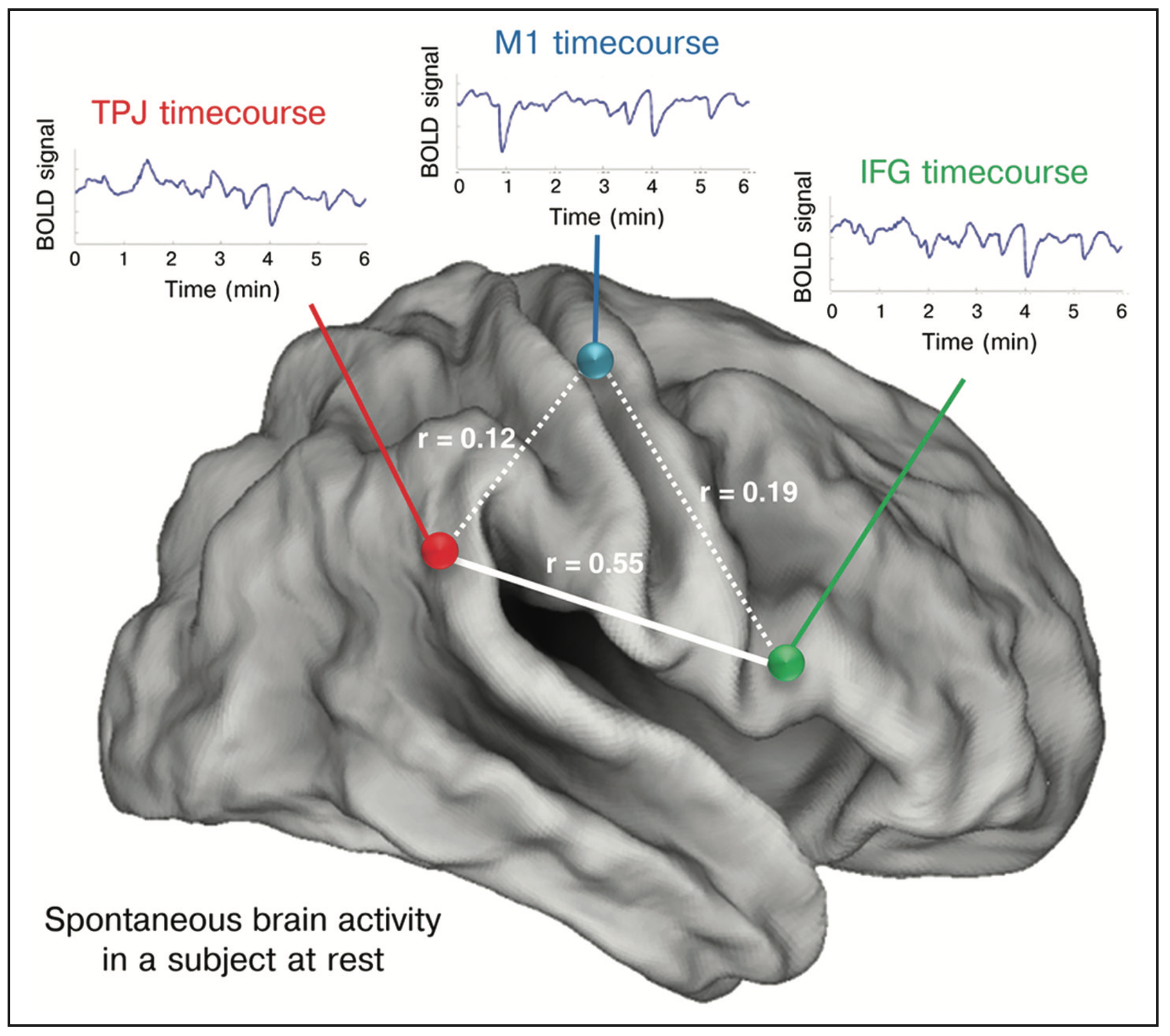
Functional Connectivity. [Gillebert et al., 2013]
Functional connectivity is defined as the temporal coincidence of spatially distant neurophysiological events.
For each participant \(i\), let \(\mathbf{y}_{ij} \in \mathbb{R}^{\mathscr T}\) be the longitudinal measurement of blood oxygen level-dependent (BOLD) signal on the region of interest \(j\), \(j = 1,2,\ldots,p\).
The functional connectivity matrix for participant \(i\) is the covariance matrix of \(\mathbf y_{i}\): \(\mathbf{\Sigma}_i = \textbf{Cov}(\mathbf{y}_i) \succeq \mathbf{0}\)
We want to link the functional connectivity matrix to the clinical outcomes using clustering methods.
K-Means Algorithm
\[\begin{align*} & \underset{\mathscr C}{\text{minimize }} \underbrace{\frac{1}{n}\sum_{j=1}^m \sum_{k \in \mathscr C_j} \big\Vert x_k - \bar x_{\mathscr C_j}\big\Vert^2}_{\text{within cluster sum of squares}} \\ &\textbf{ OR } \\ &\underset{\mathscr C}{\text{maximize}} \underbrace{\sum_{i=m} \frac{n_{\mathscr C_j}}{n}\cdot\big\Vert\bar x_{\mathscr C_j}\big\Vert^2 }_{\text{between cluster sum of squares}} \end{align*}\] Minimize the Euclidean distance between the data points to its closet centroid
Clustering Centers
\[\begin{align*} \mathbf u_j & = \mathscr E[\mathbf X \vert \mathbf X \in \mathscr C_j] \\ & = \frac{1}{n_j}\sum_{i=1}^{n_j} \mathbf x_i \cdot \delta(\mathbf x_i \in \mathscr C_j), \end{align*}\] where the centers of cluster \(\mathscr C_j\) is the average of the data points that is classified to the group \(\mathscr C_j\).
Positive Semi-Definite Matrices
Examples of Positive Semi-Definite Matrices
- \(\mathbf \psi_{2\times 2} = \begin{bmatrix} 1 & 0.5 \\ 0.5 & 1 \end{bmatrix}\)
- \(\mathbf \psi_{3\times 3} = \begin{bmatrix} 1 & 0.5 & 0.3 \\ 0.5 & 1 & 0.2 \\ 0.3 & 0.2 & 1 \end{bmatrix}\)
- \(\mathbf \psi_{p\times p} = \begin{bmatrix} x_{11} & x_{12} & \cdots & x_{1p} \\ x_{21} & x_{22} & \cdots & x_{2p} \\ \vdots & \vdots & \ddots & \vdots \\ x_{p1} & x_{p2} & \cdots & x_{pp} \end{bmatrix}\)
Visualization
A ellipsoid centered at origin is defined by the set of points \(\mathbf x \in \mathbb R^p\) such that \(\mathbf x^T \mathbf \psi \mathbf x = 1\).
Positive Semi-Definite Matrices Visualization
Formulation of K-Tensors
- let \(\mathbf \Psi\) be a random positive semi-definite matrix, and \(\mathbf \psi\) be an observed PSD matrix
- let \(\mathscr V_q(\mathbb R^p)\) be the Stiefel manifold, the set of \(p \times q\) matrices with orthonormal columns
- hyperplane can be define by \(\mathbf B \in \mathscr V_q(\mathbb R^p)\)
Definition 1: pseudo-eigenvalues of \(\mathbf \psi\) with respect to \(\mathbf B\) is defined as \[ \Lambda(\mathbf \psi, \mathbf B) := \arg\min_{\mathbf \Theta} \Vert \mathbf \psi - \mathbf B \mathbf \Theta \mathbf B^T \Vert_F^2 \]
Definition 2: projection of \(\mathbf \psi\) onto \(\mathbf B\in \mathscr V_q(\mathbb R^p)\) is defined as \[\begin{align*} \mathscr P_{\mathbf B}(\mathbf \psi) = \mathbf B \mathbf\Lambda_{\mathbf B}(\mathbf \psi) \mathbf B^\intercal \end{align*}\]
Definition 3: the hyperplane (center) that best approximates \(\mathbf \psi\) is defined as \[\begin{align} & \mathbf B(\mathbf \Psi) = \underset{{\mathbf B \in \mathscr V_p(\mathbb R^p)}}{\arg\min} \ \mathscr E \left\{ \left\Vert \mathbf \Psi - \mathscr P_{\mathbf B}\left( \mathbf \Psi \right) \right\Vert_{F}^2 \right\} \end{align}\]
K-Tensors Parametrized by \(\mathbf B\)
Algorithm:
- start with a random partition of the data
- compute the \(\mathbf B\) for each partition
- reassign all the matrix to the closest \(\mathbf B\) by
- repeat until convergence
More on K-Tensors

![]()